Robust PCA 学习笔记

Rachel Zhang

 

1. RPCA Brief Introduction

1.     Why use Robust PCA?

Solve the problem withspike noise with high magnitude instead of Gaussian distributed noise.

 

2.     Main Problem

Given C = A*+B*, where A*is a sparse spike noise matrix and B* is a Low-rank matrix, aiming at recoveringB*.

B*= UΣV’, in which U∈Rn*k ,Σ∈Rk*k ,V∈Rn*k

 

3.     Difference from PCA

Both PCA and Robust PCAaims at Matrix decomposition, However,

In PCA, M = L0+N0,    L0:low rank matrix ; N0: small idd Gaussian noise matrix,it seeks the best rank-k estimation of L0 by minimizing ||M-L||2 subjectto rank(L)<=k. This problem can be solved by SVD.

In RPCA, M = L0+S0, L0:low rank matrix ; S0: a sparse spikes noise matrix, we’lltry to give the solution in the following sections.

 

 

 

2. Conditionsfor correct decomposition

4.     Ill-posed problem:

Suppose sparse matrix A* and B*=eiejTare the solution of this decomposition problem.

1)       With the assumption that B* is not only low rank but alsosparse, another valid sparse-plus low-rank decomposition might be A1= A*+ eiejT andB1 = 0, Therefore, we need an appropriatenotion of low-rank that ensures that B* is not too sparse. Conditionswill be imposed later that require the space spanned by singular vectors U andV (i.e., the row and column spaces of B*) to be “incoherent” with the standardbasis.

2)       Similarly, with the assumption that A* is sparse as well aslow-rank (e.g. the first column of A* is non-zero, while all other columns are0, then A* has rank 1 and sparse). Another valid decomposition might be A2=0,B2 = A*+B* (Here rank(B2) <= rank(B*) + 1). Thus weneed the limitation that sparse matrix should beassumed not to be low rank. I.e., assume each row/column does not havetoo many non-zero entries (don’t exist dense row/column), to avoid such issues.

 

 

5.     Conditions for exact recovery / decomposition:

If A* and B* are drawnfrom these classes, then we have exact recovery with high probability [1].

1)       For low rank matrix L---Random orthogonal model [Candes andRecht 2008]:

A rank-k matrix B* with SVD B*=UΣV’ is constructed in this way: Thesingular vectors U,V∈Rn*k are drawnuniformly at random from the collection of rank-k partial isometries(等距算子) inRn*k. The singular vectors in U and V need not be mutuallyindependent. No restriction is placed on the singular values.

2)       For sparse matrix S---Random sparsity model:

The matrix A* such that support(A*) is chosen uniformlyat random from the collection of all support sets of size m. There is noassumption made about the values of A* at locations specified by support(A*).

[Support(M)]: thelocations of the non-zero entries in M

Latest [2] improved on the conditions andyields the ‘best’ condition.

 

 

 

3. Recovery Algorithms

6.     Formulization

For decomposition D = A+E,in which A is low rank and error E is sparse.

1)       Intuitively propose

minrank(A)+γ||E||0,    (1)

However, it is non-convex thus intractable (both of these 2are NP-hard to approximate).

2)       Relax L0-norm to L1-norm and replace rank with nuclear norm

min||A||* + λ||E||1,

where||A||* =Σiσi(A)   (2)

        This is convex, i.e., exist a uniquely minimizer.

Reason: This relaxation ismotivated by observing that ||A||* + λ||E||1 is theconvex envelop (凸包) of rank(A)+γ||E||0 over the set of (A,E) suchthat max(||A||2,2,||E||1, ∞)≤1.

Moreover, there might be circumstancesunder which (2) perfectly recovers low-rank matrix A0.[3] shows itis indeed true under surprising broad conditions.

 

 

7.     Approach RPCA Optimization Algorithm

We approach in twodifferent ways. 1st approach, use afirst-order method to solve the primal problem directly. (E.g. ProximalGradient, Accelerated Proximal Gradient (APG)), the computational bottleneck ofeach iteration is a SVD computation. 2ndapproach is to formulate and solve the dual problem, and retrieve the primalsolution from the dual optimal solution. The dual problem too RPCA canbe written as:

maxYtrace(DTY) , subject to J(Y) ≤ 1

where J(Y) = max(||Y||2,λ-1||Y||∞). ||A||x means the x norm of A.(无穷范数表示矩阵中绝对值最大的一个)。This dual problem can besolved by constrained steepest ascent.

Now let’s talk about Augmented Lagrange Multiplier (ALM) and Alternating Directions Method (ADM) [2,4].

 

7.1. General method of ALM

For the optimizationproblem

min f(X), subj. h(X)=0     (3)

we can define the Lagrangefunction:

L(X,Y,μ) = f(X)+<Y, h(x)>+μ/2||h(X)|| F2       (4)

where Y is a Lagrangemultiplier and μ is a positive scalar.

General method of ALM is:

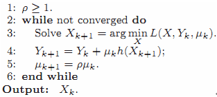
A genetic Lagrangemultiplier algorithm would solve PCP(principle component pursuit) by repeatedlysetting (Xk) = arg min L(Xk,Yk,μ), and then the Lagrangemultiplier matrix via Yk+1=Yk+μ(hk(X))

 

7.2  ALM algorithm for RPCA

In RPCA, we can define (5)

X = (A,E), f(x) = ||A||* + λ||E||1, andh(X) = D-A-E

Then the Lagrange functionis (6)

L(A,E,Y, μ) = ||A||* + λ||E||1+ <Y, D-A-E>+μ/2·|| D-A-E || F 2

The Optimization Flow isjust like the general ALM method. The initialization Y= Y0* isinspired by the dual problem(对偶问题) as it is likely to make the objective function value <D,Y0*> reasonably large.

 

Theorem 1.  For algorithm 4, any accumulation point (A*,E*) of (Ak*, Ek*)is an optimal solution to the RPCA problemandthe convergence rate is at least O(μk-1).[5]

 

Inthis RPCA algorithm, a iteration strategy is adopted. As the optimizationprocess might be confused, we impose 2 well-known facts: (7)(8)

 

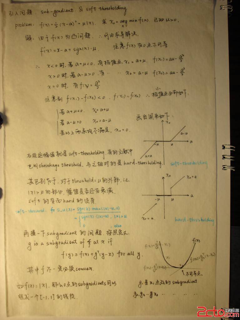
Sε[W] = arg minX ε||X||1+ ½||X-W||F2       （7）

U Sε[W] VT = arg minX ε||X||*+½||X-W||F2        （8）

which is used in the abovealgorithm for optimization one parameter while fixing another. In thesolutions, Sε[W] is the soft thresholding operator. Here I will impose the problemto speculate this. (To facilitate writing formulation and ploting, I use amanuscript. )

 

 

 

 

 

 

 

 

 

Now we utilize formulation (7,8) into RPCA problem.

For the objective function (6) w.r.t get optimal E, wecan rewrite the objective function by deleting unrelated component into:

f(E) = &la

补充：软件开发 , C++ ,